9 Unsupervised learning: Clustering

! pip install scikit-learn-extra rdkit

!mkdir data/
!wget https://raw.githubusercontent.com/schwallergroup/ai4chem_course/main/notebooks/04%20-%20Unsupervised%20Learning/data/unknown_clusters.csv -O   data/unknown_clusters.csv
!wget https://raw.githubusercontent.com/schwallergroup/ai4chem_course/main/notebooks/04%20-%20Unsupervised%20Learning/utils.py -O utils.py

from sklearn.datasets import make_blobs
import numpy as np
from sklearn.decomposition import PCA
from sklearn.cluster import KMeans, DBSCAN
from sklearn_extra.cluster import KMedoids
from sklearn.metrics import silhouette_score
import matplotlib.pyplot as plt
import pandas as pd

from rdkit import DataStructs
from rdkit.ML.Cluster import Butina
from sklearn.metrics import pairwise_distances

from rdkit.Chem import AllChem, Descriptors, MolFromSmiles, rdMolDescriptors
from rdkit import Chem
from rdkit.Chem import Draw

from utils import plot_3d, plot_2d

Clustering

Clustering is a powerful unsupervised learning technique that aims to group similar data points together based on their features or attributes. This technique can be used to gain insights into the underlying structure of large and complex datasets, and to identify patterns and relationships that may not be immediately apparent.

In this notebook, we will explore four different clustering algorithms:

KMeans
KMedoids
DBSCAN
Butina clustering

These algorithms are widely used in a variety of fields, including chemistry, and can help researchers better understand data and make informed decisions. We will start by applying each algorithm to a synthetic clustered dataset, and evaluate their performance using different clustering metrics.

After analyzing the clustering algorithms on the synthetic dataset, you will apply them to a real-world chemistry dataset to uncover the true number of clusters using metrics like silhouette and inertia. By the end of this notebook, you will have a better understanding of how clustering works and how to apply different clustering algorithms to real-world problems.

Let’s start by generating a synthetic clustering dataset using the make_blobs function from scikit-learn.

The make_blobs function generates a set of random data points with a Gaussian distribution. The data points are generated in clusters, with each cluster representing a group of points that have similar features. The function returns arrays X and y, with X containing the coordinates of each data point, and y containing the labels of each data point, indicating which cluster it belongs to.

By using different values for the parameters of the make_blobs function, we can generate synthetic datasets with different characteristics of the clusters, different numbers of clusters, features, and standard deviations. We can use these datasets to evaluate different clustering algorithms.

# Generate synthetic clustered data
n_clusters = 4
n_features = 512

# Define custom cluster standard deviations
cluster_stds = [0.5, 1.5, 1, 2.0]
n_samples = [200, 300, 100, 150]
cluster_centers = np.random.randint(-5, 5, size=(n_clusters, n_features))

X, y = make_blobs(n_samples=n_samples, centers=None, cluster_std=cluster_stds, n_features=n_features, center_box=(-1, 1))

# Convert the data to binary to emulate molecular fingerprints
X_binary = np.where(X > 0, 1, 0)  # Binary data

# Get the coordinates for plotting using PCA
pca = PCA(n_components=3)
coords = pca.fit_transform(X_binary)

KMeans

KMeans is one of the most popular clustering algorithms in machine learning. It works by partitioning a dataset into k distinct clusters, with k predetermined by the user. KMeans iteratively assigns each data point to the nearest centroid (the center of the cluster), and then updates the centroid based on the mean of all the data points assigned to it. The algorithm continues to iterate until the centroids no longer move significantly or a predetermined number of iterations is reached.

KMeans is widely used in various applications, including image segmentation, market segmentation, and data mining. It is a simple yet powerful algorithm that can efficiently cluster large datasets. However, its performance can be highly dependent on the initialization of the centroids, and it may not work well with datasets that have non-spherical or overlapping clusters.

# Defining KMeans method with n_clusters
kmeans = KMeans(n_clusters=n_clusters, n_init=10, init='k-means++')
kmeans.fit(X_binary)

We can plot the result of KMeans clustering on our dataset by visualizing the data in the lower-dimensional space and coloring the data points based on the clusters. We can see that KMeans was able to effectively cluster the data points into four distinct clusters, which closely match the actual clusters generated by the make_blobs function.

fig, (ax1, ax2) = plt.subplots(1, 2, figsize=(12, 5))

plot_2d(coords, y, title="Actual Clusters", ax=ax1)
plot_2d(coords, kmeans.labels_, title="KMeans Predicted Clusters", ax=ax2)

plt.show()

Sometimes, looking at the data in 2D may not be enough to fully understand the underlying structure and patterns. If that’s the case, we can use the third PCA component to plot the data in 3D.

plot_3d(coords, labels=kmeans.labels_, title="KMeans clustering")

KMedoids

KMedoids is a clustering algorithm similar to KMeans, with some key differences. Like KMeans, KMedoids is an unsupervised learning algorithm that aims to partition a dataset into k predefined distinct clusters. However, unlike KMeans, KMedoids uses medoids (i.e., the most centrally located data point in each cluster) instead of centroids as the representative point for each cluster. This makes KMedoids more robust to noise and outliers, and allows it to handle non-spherical and non-convex clusters. The central point of the cluster with KMedoids has to be the point from the dataset, while KMeans uses any point in the space.

This difference is illustrated in the image:

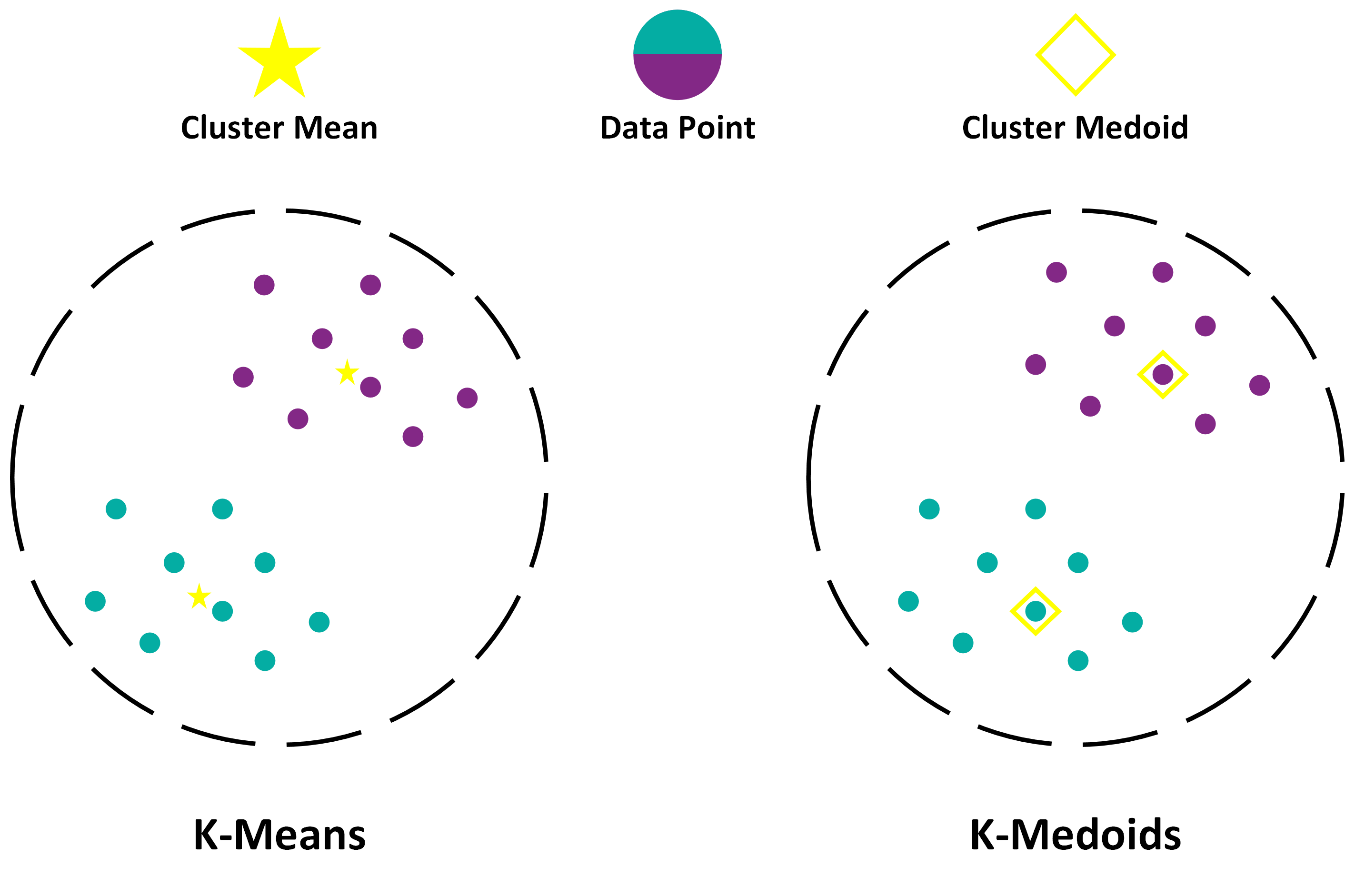
K-means typically uses the Euclidean distance metric, while K-medoids work with any distance metric, making it more versatile and adaptable to different types of datasets.

Make sure to try different metrics for the KMedoids algorithm and see how the clustering changes. Available options include Jaccard, cityblock, cosine, and others.

kmedoids = KMedoids(n_clusters=n_clusters, random_state=42, init='k-medoids++', metric='euclidean', max_iter=50000)
kmedoids.fit(X_binary)

fig, (ax1, ax2) = plt.subplots(1, 2, figsize=(12, 5))

plot_2d(coords, y, title="Actual Clusters", ax=ax1)
plot_2d(coords, kmedoids.labels_, title="KMedoids Predicted Clusters", ax=ax2)

plt.show()

plot_3d(coords, labels=kmedoids.labels_, title="KMedoids clustering")

DBSCAN (Density-Based Spatial Clustering of Applications with Noise)

DBSCAN is a clustering algorithm that groups data points based on their density. It can find arbitrarily shaped clusters and is robust to noise. Unlike K-means and K-medoids, DBSCAN does not require specifying the number of clusters beforehand. The key idea behind DBSCAN is that a cluster is a dense region of points separated from other dense regions by areas of lower point density.

DBSCAN requires two parameters:

eps (epsilon): The maximum distance between two points to be considered as neighbors.
min_samples: The minimum number of points required to form a dense region (core points).

The algorithm works by defining a neighborhood around each data point and grouping together points that are close to each other based on the eps parameter. If a neighborhood contains at least min_samples points, the point is considered as a core point. Points that are not core points but are reachable from a core point belong to the same cluster as the core point. Points that are not reachable from any core point are treated as noise.

dbscan = DBSCAN(eps=0.5, min_samples=5, metric='jaccard')
dbscan.fit(X_binary)

fig, (ax1, ax2) = plt.subplots(1, 2, figsize=(12, 5))

plot_2d(coords, y, title="Actual Clusters", ax=ax1)
plot_2d(coords, dbscan.labels_, title="DBSCAN Predicted Clusters", ax=ax2)

plt.show()

Butina Clustering Algorithm

The Butina clustering algorithm is an unsupervised clustering method designed specifically for handling large datasets with binary features. It is particularly useful in chemoinformatics for clustering molecular fingerprints, which are binary representations of molecular structures. Butina clustering algorithm is a single-linkage hierarchical clustering method that merges clusters based on a user-defined similarity threshold (cutoff).

One of its main advantages over other clustering methods is the ability to work well with binary data and non-Euclidean distance metrics, like Jaccard.

To set the cutoff parameter for Butina clustering, follow these steps:

Calculate the pairwise distances (using Jaccard or another suitable metric) for your dataset.
Visualize the distribution of distances by plotting a histogram.
Analyze the histogram and choose a cutoff value that corresponds to a reasonable threshold for distinguishing between similar and dissimilar data points.

Once you have chosen an appropriate cutoff value, use it as the input parameter for the Butina clustering algorithm. You can experiment with different cutoff values to find the one that produces the most satisfactory clustering results for your data.

distances = pairwise_distances(X_binary.astype(bool), metric='jaccard')

plt.hist(distances.flatten(), bins=50)
plt.xlabel("Jaccard Distance")
plt.ylabel("Frequency")
plt.show()

class ButinaClustering:
    def __init__(self, cutoff=0.8, metric='jaccard'):
        self.cutoff = cutoff
        self.metric = metric

    def fit(self, x):
        """
        Perform Butina clustering on a set of fingerprints.

        :param x: A numpy array of binary data
        :return: self
        """
        # Calculate the distance matrix
        distance_matrix = []
        x = x.astype(bool)
        for i in range(1, len(x)):
            distances = pairwise_distances(x[i,:].reshape(1, -1), x[:i,:], metric=self.metric)
            distance_matrix.extend(distances.flatten().tolist())

        # Perform Butina clustering
        clusters = Butina.ClusterData(distance_matrix, len(x), self.cutoff, isDistData=True)
        self.clusters = clusters

        # Assign cluster labels to each data point
        cluster_labels = np.full(len(x), -1, dtype=int)
        for label, cluster in enumerate(clusters):
            for index in cluster:
                cluster_labels[index] = label

        self.labels_ = cluster_labels


    def fit_predict(self, x):
      self.fit(x)
      return self.labels_

butina = ButinaClustering(cutoff=0.65, metric='jaccard')
butina.fit(X_binary)

len(butina.clusters)

fig, (ax1, ax2) = plt.subplots(1, 2, figsize=(12, 5))

plot_2d(coords, y, title="Actual Clusters", ax=ax1)
plot_2d(coords, butina.labels_, title="Butina Predicted Clusters", ax=ax2)

plt.show()

In the next section, we will evaluate how clustering metrics like inertia and silhouette score can help us uncover the optimal number of clusters when using KMeans or KMedoids algorithm.

Inertia

Inertia is the sum of squared distances between each data point and its assigned cluster centroid. It is a measure of how tightly grouped the data points are within each cluster. A lower inertia value indicates that the data points within a cluster are closer to their centroid, which is desirable. However, inertia can be sensitive to the number of clusters, as increasing the number of clusters will generally reduce the inertia. Therefore, selecting the optimal number of clusters based on inertia alone can lead to overfitting.

Silhouette Score

The silhouette score is a measure of how similar a data point is to its own cluster compared to other clusters. The silhouette score ranges from -1 to 1. A high silhouette score indicates that data points are well-matched to their own cluster and poorly matched to neighboring clusters. A negative silhouette score implies that data points might have been assigned to the wrong cluster. The silhouette score can be more robust than inertia in determining the optimal number of clusters, as it considers both cohesion (how closely related the data points within a cluster are) and separation (how distinct the clusters are from each other).

To compare inertia and silhouette scores and determine the optimal number of clusters for the data, you can follow these steps:

Loop through a range of cluster numbers (e.g., 2 to 10) and fit the clustering algorithms (KMeans, KMedoids, etc.) for each number of clusters.
Calculate and store the inertia and silhouette scores for each clustering model and each number of clusters.
Plot the inertia and silhouette scores as a function of the number of clusters.
Examine the plots to determine the optimal number of clusters. For the inertia plot, look for an “elbow” point, where the rate of decrease in inertia starts to level off. For the silhouette plot, look for the highest silhouette score.

n_clusters = 4
algorithms = {
    'KMeans': KMeans(n_clusters=n_clusters, n_init=10, init='k-means++', random_state=42),
    'KMedoids': KMedoids(n_clusters=n_clusters, init='k-medoids++', metric='jaccard', random_state=42)
}

def plot_inertia_and_silhouette(data, algorithms, min_clusters, max_clusters):
    
    for name, algorithm in algorithms.items():
        fig, (ax1, ax2) = plt.subplots(1, 2, figsize=(12, 5))
        fig.suptitle(f'{name}')

        inertia = []
        silhouette_scores = []
        for n_clusters in range(min_clusters, max_clusters + 1):
            algorithm.set_params(n_clusters=n_clusters)
            labels = algorithm.fit_predict(data)
            inertia.append(algorithm.inertia_)
            silhouette_scores.append(silhouette_score(data, labels))
        
        ax1.plot(range(min_clusters, max_clusters + 1), inertia, label=name)
        ax2.plot(range(min_clusters, max_clusters + 1), silhouette_scores, label=name)
    
    ax1.set_xlabel("Number of clusters")
    ax1.set_ylabel("Inertia")
    ax1.legend()
    
    ax2.set_xlabel("Number of clusters")
    ax2.set_ylabel("Silhouette Score")
    ax2.legend()
    
    plt.show()

min_clusters = 2
max_clusters = 10

plot_inertia_and_silhouette(X_binary.astype(bool), algorithms, min_clusters, max_clusters)

Now it’s your turn to find the optimal number of clusters in a chemical dataset using KMeans or KMedoids algorithms and the inertia vs. silhouette metrics. Using the plot_inertia_and_silhouette function estimate the correct number of clusters in the unknown_clusters dataset. Steps: - Read the dataset under data/unknown_clusters.csv - Featurize smiles using Morgan fingerprints - Run the plot_inertia_and_silhouette function to estimate the optimal number of clusters

# YOUR CODE
data = 
# ...

Once you’ve estimated the number of clusters, update the N_CLUSTERS variable with the correct number and run a visualization function to see some of the molecules in your clusters.

# YOUR CODE
N_CLUSTERS =

import numpy as np
from sklearn.cluster import KMeans
from sklearn_extra.cluster import KMedoids
from rdkit import Chem
from rdkit.Chem import Draw

# Perform clustering using KMeans and KMedoids
n_clusters = N_CLUSTERS
kmeans = KMeans(n_clusters=N_CLUSTERS, n_init=10, random_state=42).fit(X)
kmedoids = KMedoids(n_clusters=n_clusters, init='k-medoids++', metric='jaccard', random_state=42).fit(X.astype(bool))


# Function to select a few representative molecules from each cluster
def plot_representative_molecules(labels, smiles, n_clusters, n_molecules=5):
    for i in range(n_clusters):
        cluster_indices = np.where(labels == i)[0]
        molecules = [Chem.MolFromSmiles(smile) for smile in smiles]
        cluster_molecules = [molecules[idx] for idx in cluster_indices]

        # Select the first n_molecules from the cluster
        selected_molecules = cluster_molecules[:n_molecules]

        # Plot the selected molecules
        img = Draw.MolsToGridImage(selected_molecules, molsPerRow=n_molecules, subImgSize=(200, 200))
        print(f"Cluster {i+1}:")
        display(img)

# Plot the representative molecules for KMeans
print("KMeans Clusters:")
plot_representative_molecules(kmeans.labels_, data['smiles'], N_CLUSTERS)

# Plot the representative molecules for KMedoids
print("KMedoids Clusters:")
plot_representative_molecules(kmedoids.labels_, data['smiles'], N_CLUSTERS)